





Speculative decoding (SD) is a popular technique for accelerating large language model (LLM) inference without any loss in quality. LLM inference generates one token at a time. SD instead uses a smaller draft model to propose multiple tokens, which are then verified by the large target model in a single timestep. Because more than one token can be accepted per step, this speeds up generation.
SD achieves its speedup by exploiting the tradeoff between the compute and memory bandwidth of a GPU. Batching multiple requests improves GPU utilization, but the operating regime depends on the batch size (BS):
- At small BS, inference is memory bandwidth-bound: the cost of loading LLM weights from HBM into SRAM dominates.
- At large BS, inference becomes compute-bound: the matrix multiplications of LLM weights against many request tokens dominate.
The time spent in SD has two main components:
Time in SD = Time to draft tokens (small draft model) + Time to verify draft tokens (large target model)
Draft models are much cheaper to run. If the draft produces K tokens, the target model must process BS × (K+1) tokens, which makes verification the bottleneck since it does K+1 times more computation for a given BS. On modern GPUs, the compute units are typically about two orders of magnitude faster than memory bandwidth, so during memory bandwidth-bound, small-BS inference, the compute units sit largely idle. SD leverages this gap by pushing K+1 times more tokens through the target model during verification, using compute that would otherwise be wasted.
Challenges in speculative decoding
Dynamic batching in production
As batch size grows, ordinary LLM inference becomes increasingly compute-bound, leaving no idle compute for SD to exploit. In this regime, SD can actually be slower than ordinary inference. This limits SD in production systems, where BS is rarely small and changes dynamically.
Reinforcement learning (RL)
RL alternates between a training phase, which updates model weights, and a rollout phase, which generates data and reward signals to train on. The rollout phase is the main bottleneck and can consume up to 85% of resources. Since scaling RL is an important avenue for improving model intelligence, accelerating RL rollout inference is an important problem to solve.
However, RL with reasoning models produces a long-tail distribution: a single request in a batch can keep generating for a very long time, stalling the rest of the batch and wasting resources. SD would help with these long-tail generations, but because it hurts throughput at high BS, its overall utility in a full deployment is limited.
Together, these challenges point to the same requirement: a better SD system should control the optimal K based on hardware constraints, so that it remains useful in full production systems and large-scale RL rollouts.
Dynamic speculative decoding
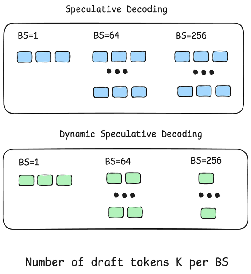
This is where hardware-aware dynamic SD (DSD) comes in. DSD improves on standard SD by making the number of draft tokens adaptive. In SD, K is fixed; in DSD, the optimal K is chosen based on the interaction between the model and the hardware. DSD increases K when inference is memory bandwidth-bound and decreases it when inference is compute-bound.
For dense models, this generally means a higher K at low BS and a lower K at high BS, with the optimal K decreasing monotonically as BS grows. For MoE (Mixture-of-Experts) models, the optimal K is non-monotonic in BS:
- At low BS, optimal K starts low because verification loads additional experts.
- At mid BS, optimal K increases because almost all experts are already loaded, so verification adds little extra expert loading.
- At high BS, optimal K decreases again, just like a dense model, because the computation is now compute-bound.
For a deeper treatment of these mechanics, see our previous blog post on the interaction of SD with MoEs.
So, how do we find the optimal number of draft tokens? We need to understand the marginal contribution of going from K to K+1 draft tokens. The computational cost of processing one draft token is the same regardless of its position — the first and last draft tokens cost the same. Its contribution to the Acceptance Length (AL), however, depends heavily on position: it decays exponentially, so earlier tokens are far more likely to be accepted than later ones. We therefore need a metric that captures this tradeoff when adding one more draft token.
Existing DSD work, such as TurboSpec, uses goodput as this metric. We use goodput too, but simplify it to:
goodput = AL / ITL
AL is the acceptance length, and ITL is the inter-token latency (largely the sum of the draft and verify times). This captures the tradeoff between the marginal contribution of K draft tokens to AL and the wall clock cost, with a higher value implying a better speedup. This simple formulation makes DSD easy to adapt to future model architectures, and since ITL already encapsulates the combined impact of all operations, there's no need to profile each component individually and recombine them. We run offline profiling to measure AL and ITL, find the optimal K, and store it as a lookup table used at runtime. This offline table solves the cold-start problem and is extensible: it can incorporate live AL and ITL statistics from the engine's runtime metrics, allowing DSD to adapt to changing workloads.
Results
We compare three configurations: vanilla (no speculative decoding), fixed-K SD (our SD baseline, implemented with an EAGLE draft head at a fixed K=3), and DSD (dynamic K) on the MT-Bench dataset with the number of samples upsampled to 20 * BS, which implies 20 waves of BS being used.
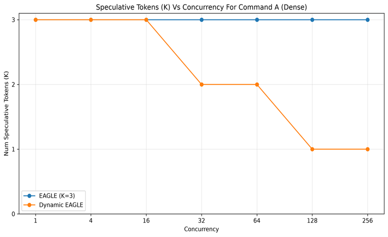
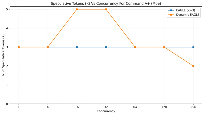
We profiled the optimal K selected by DSD for both Command A (Dense) and Command A+ (MoE). The empirical results validate the trends described above: for the dense model, the optimal K decreases monotonically as BS increases, whereas for the MoE model it does not — Command A+ can reach a higher optimal K at mid BS.
We also benchmark TOPS/user (token output per second, per user). For Command A (Dense), the gains from DSD are clear across the whole BS range:
- At low BS, DSD matches the speedup of SD (K=3).
- At high BS (64/128), DSD is faster than both SD and the vanilla model.
- At very high BS (256), DSD matches vanilla TOPS — even though SD regresses at BS 128 and 256.
Concretely, DSD is ~23% faster than SD at both BS 128 and BS 256. It is also 7.5% faster than vanilla at BS 128 and 1.82% faster at BS 256, whereas SD regresses relative to vanilla in this range. In other words, DSD captures the SD speedup where it helps and gracefully falls back toward vanilla performance where fixed-K SD would otherwise hurt.
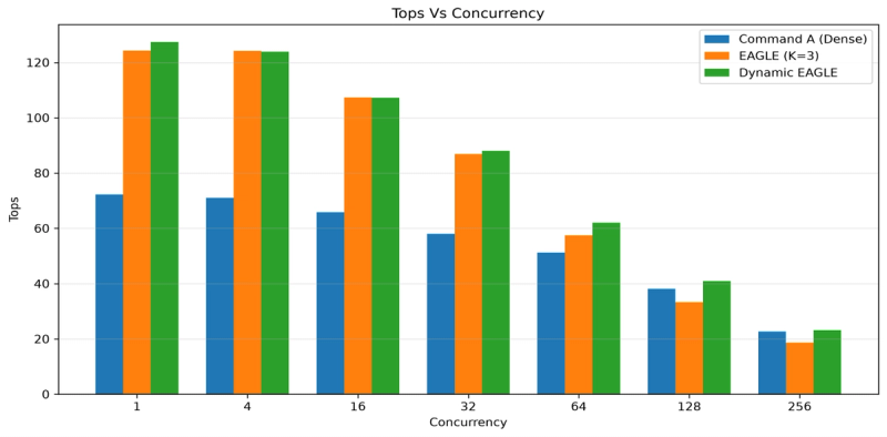
For Command A+ (MoE), SD and DSD deliver similar speedups. This is because DSD selects K=3 for most of the BS range — matching fixed-K SD — except between BS 16 and 32, where it selects K=5. That higher K did not translate into additional speedup, most likely because the EAGLE head is trained for a single timestep but reused across K > 1 timesteps, so acceptance is not high enough to yield a boost. We expect more recent methods, such as EAGLE-3 or DFlash, to show clearer gains in this scenario.
Our contributions to vLLM
Earlier this year, we contributed this optimization to vLLM (pull request; see vLLM docs for usage). While the idea of DSD is not new and a naive implementation would be simple, the real challenge was adopting it inside a highly optimized inference framework like vLLM. vLLM ships many optimizations — such as async scheduling and full CUDA Graph — and DSD has to be compatible with all of them to fully extract vLLM's efficiency. We discuss the two most important below.
Compatibility with async scheduling
An inference framework first schedules requests (CPU work) and then runs model inference (GPU work). Historically the GPU was the bottleneck, but as production-grade GPUs get faster, the CPU scheduling overhead becomes relatively larger — the GPU finishes early and waits for the next batch to be scheduled. To address this, vLLM introduced asynchronous scheduling, which hides scheduler latency by overlapping the scheduler for timestep T+1 (on CPU) with the model runner for timestep T (on GPU). This minimizes scheduler overhead on the CPU.
Crucially, the scheduler at T+1 runs without the model runner's output from T, which is still executing in parallel. This works because the scheduler operates purely on counts and placeholders on the CPU, one step ahead; the actual token values live on the GPU and are consumed one step later by the model runner via a GPU-side scatter. Only lightweight counts (placeholders and token counts) cross the process boundary, asynchronously.
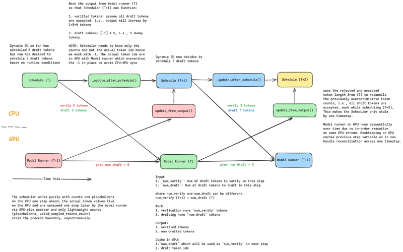
The scheduler tells the model runner how many draft tokens to generate, as well as how many draft tokens from the previous timestep to verify in the current one. DSD breaks the assumption that the same number of draft tokens is generated and verified at every timestep, which changes the bookkeeping in both the scheduler and the model runner.
The diagram below illustrates DSD under async scheduling across timesteps (zoom in to read it). Here, the system drafts five tokens up to T-1, shifts to three tokens at T, and then seven tokens at T+1.
Compatibility with full CUDA Graph
A model forward pass launches many CUDA kernels, and each kernel launch incurs CPU overhead. As modern production-grade GPUs get faster, this per-launch overhead — accumulated across many kernels — becomes a significant fraction of total inference time. Full CUDA Graph (FCG) eliminates it by capturing all kernel launches during warmup and replaying them as a single graph launch instead of many individual ones.
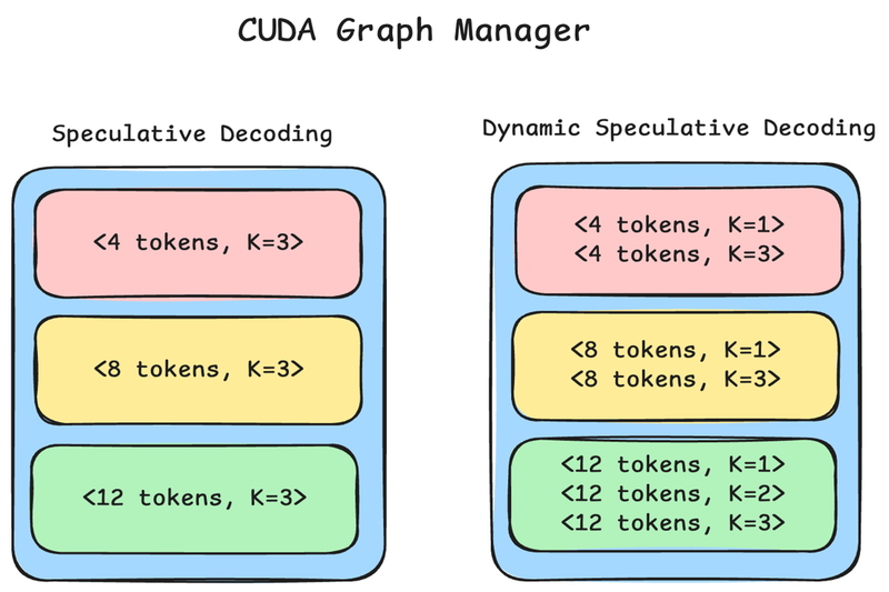
vLLM provides FCG support for decode requests by capturing tuples of <number of tokens in a batch, fixed K>. DSD extends this to capture <number of tokens in a batch, different optimal K>, recording more combinations so that changing K at runtime still hits a captured CUDA Graph (pull request).
The diagram below shows an example with max K=3. In that example with eight tokens in a batch, standard SD captures only <8 tokens, K=3>, whereas DSD captures every valid K such that the number of tokens is divisible by K+1—i.e., <8 tokens, K=1> and <8 tokens, K=3>. Divisibility by K+1 implies every request in the batch is a decode request, which is what routes to FCG in vLLM.
Acknowledgements
On the Cohere side, thank you to Acyr Locatelli and Bharat Venkitesh for providing technical support throughout this work. We extend special thanks to Lucas Wilkinson (Red Hat) and Benjamin Chislett (Nvidia) for their discussions and reviews of the vLLM PRs.