Why MoE models get more from speculative decoding

Background

Large Language Models generate text one token at a time. Each token requires a full forward pass through the model, making generation inherently slow. Speculative decoding (SD) attacks this bottleneck: a small, fast “draft” model guesses the next tokens, and the full “target” model verifies all $K+1$ of them in a single forward pass. When the guesses are right, you get multiple tokens for nearly the cost of one.

Mixture-of-Experts (MoE) models add an interesting twist. Each token only activates a small subset of the model’s parameters — called “experts” — making individual tokens cheap. But during verification, $K+1$ tokens may each route to different experts, potentially loading far more weights from memory than a single-token decode would. Does this extra loading erase the speedup that speculative decoding is supposed to deliver?

Recent work by MoESD predicts that the answer is nuanced: MoE’s low arithmetic intensity creates a non-monotonic speedup curve, where gains first increase with batch size before declining.

In this post, we validate this prediction on our production MoE models and extend the analysis in two directions. First, we examine temporal correlation in expert routing — a structural property of MoE models documented in prior work — and quantify its impact on SD verification cost. Second, we uncover a distinct mechanism behind the surprisingly high speedup at BS=1, where fixed-overhead amortization plays a role that routing analysis alone cannot explain. Finally, we also draw out concrete design implications for co-optimizing model sparsity and speculative decoding.

Observing the non-monotonic speedup curve

In LLM inference, the inference system batches multiple concurrent requests so that their decode steps execute together in a single forward pass — the number of requests processed in parallel is the *batch size* (BS). Because LLM decode is memory-bandwidth-bound at small BS and becomes compute-bound at large BS, the batch size fundamentally shapes how much benefit speculative decoding can deliver. Using vLLM, we benchmarked SD speedup across batch sizes for both a dense and a MoE model.

Dense baseline (Command A, 111B). Speedup vs. batch size shows monotonic decrease — gains are highest at low BS where the model is bandwidth-bound.

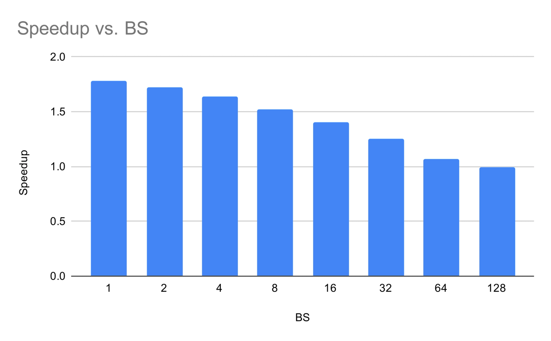
Cohere MoE + SD $K=3$. Speedup first increases then declines — the non-monotonic shape predicted by MoESD. The gain at BS=1 is unusually high; we revisit this anomaly in a later section.

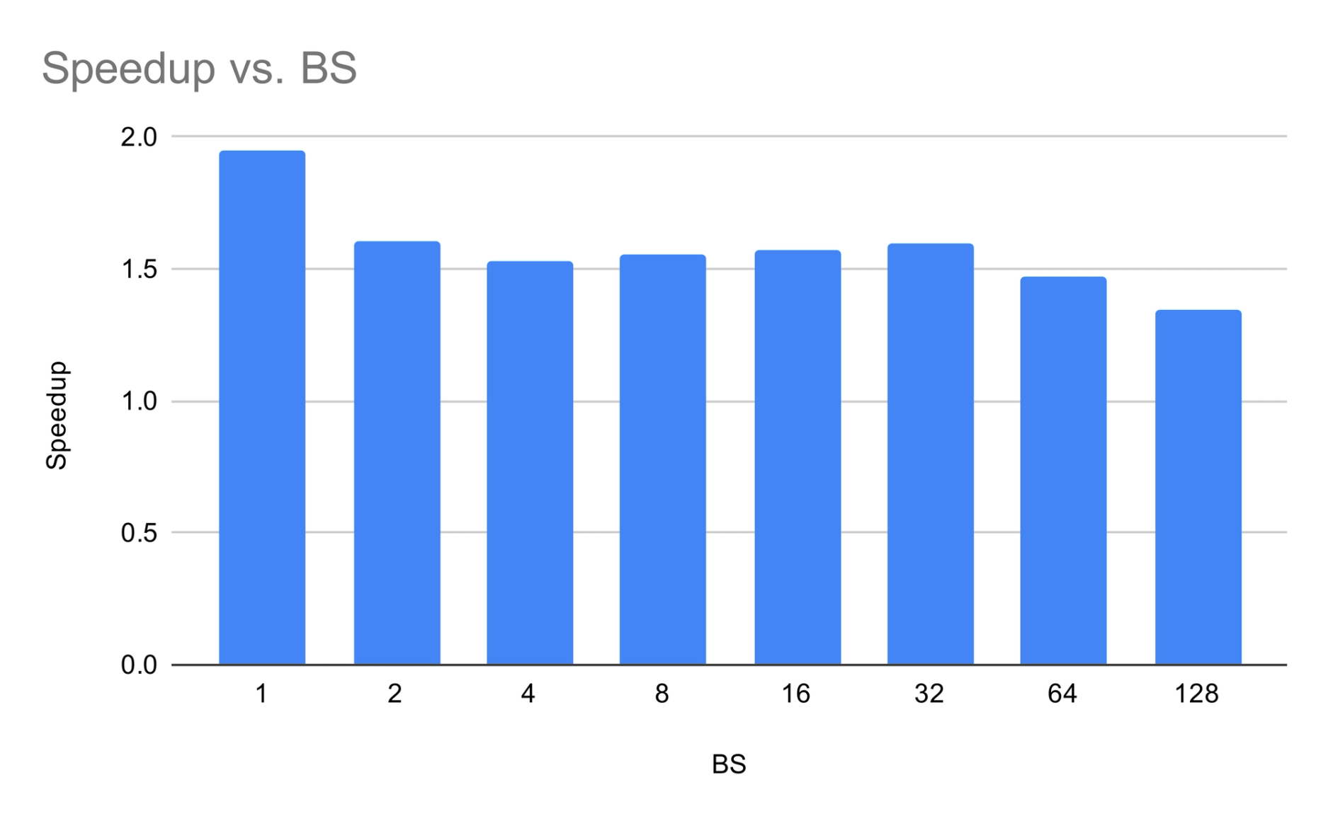
The contrast is striking: where the dense model’s SD gains monotonically decay, the MoE model exhibits a sweet spot at moderate batch sizes. What creates this sweet spot, and why does BS=1 stand out?

Why MoE creates a sweet spot: arithmetic intensity

The key to the non-monotonic curve lies in arithmetic intensity. For a MoE layer with N total experts, where each token selects $k$ of them (top-k routing), processing $T$ tokens with $S$ shared experts gives an arithmetic intensity of:

When $S=0: AI=Tk/N$. Sparsity (low $k/N$) keeps $AI$low, pushing the layer deeper into the bandwidth-bound regime at any given $T$.

This creates three batch-size regimes for SD, as analyzed in MoESD:

Low BS — partial expert loading. The model is memory-bandwidth-bound, but decode doesn’t yet load all experts. Verification adds extra expert weight loading on top of decode cost, limiting SD gains.

Moderate BS — the sweet spot. Both decode and verification load nearly all experts anyway — verification adds almost no extra weight loading. Because $AI$remains low (thanks to sparsity), the model stays bandwidth-bound, making verification tokens nearly free. SD gains peak here.

High BS — compute-bound. Arithmetic intensity exceeds the machine’s ops-to-byte ratio. Every extra verification token costs proportional compute, and SD gains vanish.

Sparser models (lower $k/N$) stay bandwidth-bound longer, pushing the sweet spot to higher batch sizes.

Connecting to SD speedup

Following MagicDec and MoESD, the SD speedup is dominated by the verification cost ratio $T_t(K + 1)/T_t(1)$. Draft overhead is typically negligible. For $K=3$, the key metric is:

As this approaches 1 (verification ≈ free), speedup approaches the theoretical maximum of $AL$ (acceptance length). The remaining sections measure and model this ratio via expert overlap analysis and Amdahl’s Law.

Co-designing model sparsity and speculation

The three-regime analysis yields a concrete design principle: for a given target batch size, the sparsity ratio $k/N$ determines whether the model operates in the bandwidth-bound sweet spot or crosses into compute-bound territory where SD gains vanish.

Sparser models (lower $k/N$) stay bandwidth-bound to higher batch sizes, widening the sweet spot. Denser models hit the compute-bound regime earlier. This means sparsity is not just a parameter-efficiency knob — it directly controls how much benefit speculative decoding can deliver at a given target BS load.

The shared-to-routed expert ratio adds a second lever: shared experts reduce verification cost at low BS (by lowering the fraction of forward-pass time spent on routed expert weight loading), but raise the effective $k/N$, pushing the compute-bound transition earlier. In the limit, a model that shares all experts is equivalent to a dense model, with no sweet spot at all.

For systems where the target BS is known at design time, these two knobs can be set accordingly:

High target BS — maximize SD benefit by:

1. Lowering $k/N$: fewer active experts per token keeps arithmetic intensity low and the model bandwidth-bound even at large batch sizes.

2. Increasing the routed-to-shared expert ratio: more routed (fewer shared) experts keep the effective $k/N$ low, preserving the bandwidth-bound regime.

Low target BS — the calculus shifts: shared experts are beneficial because they reduce the fraction of forward-pass time spent on routed weight loading, making verification cheaper. The model stays bandwidth-bound regardless due to the small batch size.

Expert routing and verification cost

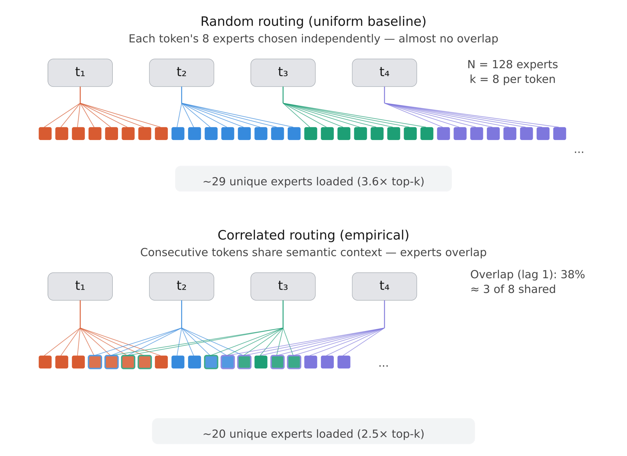
The arithmetic intensity framework explains the shape of the speedup curve, but predicting the actual verification cost requires understanding how experts are shared across tokens. If consecutive tokens during verification route to the same experts, fewer unique weights need to be loaded from memory.

Temporal correlation in expert routing — the tendency for adjacent tokens to activate overlapping sets of experts — has been documented as a structural property of MoE models. Here we study this phenomenon in the SD verification setting, quantifying its effect on verification cost using a modified version of `enable_return_routed_experts` API in vLLM to capture per-token expert routing decisions on the MT-Bench dataset."

Notation and baselines

• $N$represents number of experts per MoE layer

• $k$ represents experts selected per token (top-k)

• $L$ represents number of MoE layers

• $experts(t)$represents set of $k$ expert indices chosen for token $t$

• $p_e$ represents $\text{P(expert } e \text{ selected for a random token)}$, estimated from data

In a MoE layer, a learned router selects $k$ experts (out of $N$) per token. Only the selected experts’ weights are loaded from HBM to SRAM and applied. For SD verification, the key question is: how many unique experts must be loaded for all $K+1$ tokens?

Since each token selects exactly $k$ experts:

We compare routing statistics under three assumptions:

1. Uniform baseline — all experts equally likely $p_e = k/N$, tokens independent.

2. Independence baseline — empirical pe from data, but tokens are still independent. Captures non-uniform popularity but no temporal correlation.

3. Empirical — measured directly from consecutive tokens, preserving temporal correlation between adjacent tokens.

The gap between the independence baseline and the empirical measurement isolates the effect of temporal correlation — the mechanism that makes SD verification cheaper than the baselines predict.

Expert selection probabilities

Our model selects $k=8$ from $N=128$ experts per token. Individual layers have clear favorites — the most popular expert in a layer can be up to $10\times$ the uniform baseline $(p_{\text{uniform}} = k/N = 0.0625)$. This skewness means expert activation saturates faster with batch size, benefiting SD by reducing the unique expert count during verification.

Expected active experts vs. batch size

For SD with $K=3$, the key row is BS=4: 25.4 empirical vs. 29.1 uniform. Real routing concentrates experts. The ratio of Empirical/Uniform decreases and then recovers as BS increases — a curve that mirrors the SD gain profile for MoE.

Expert overlap between adjacent tokens

At step 1, 38% overlap (3.0 of 8 experts shared) is well above the independence baseline (11.8%) and uniform floor (6.3%). Correlation decays with distance but remains 2–4× above the independence prediction at step 4. This level of temporal correlation is consistent with the routing consistency patterns observed in this paper and has direct implications for SD: the more experts are shared between consecutive verification tokens, the fewer unique weights must be loaded.

Per-layer variation (step 1): Mid-network layers show the strongest overlap (~0.50), while early layers (~0.32) and final layers (~0.25) show less. Early layers haven’t developed strong semantic routing; final layers show reduced correlation as the model converges on the output distribution.

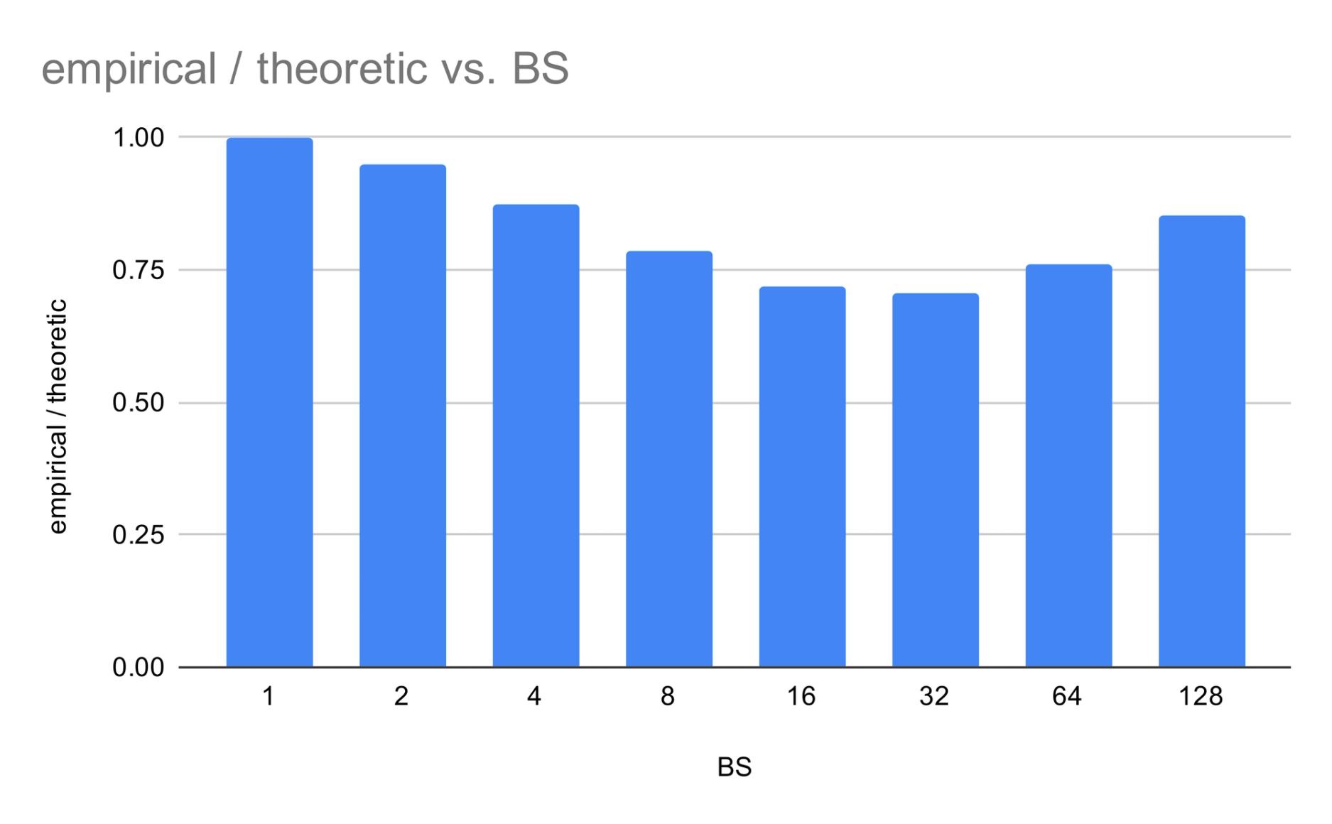
Verification cost: unique experts for $K=3$

Temporal correlation reduces unique experts by 20–31% vs. the independence baseline. Verifying four tokens activates ~2.5× top-k (not the 3.2–3.6× the baselines predict).

Generalization across data domains

We validated 13 Spec-Bench categories and seven languages from Aya Human Annotated. Expert overlap ratio at step 1:

Expert overlap is a structural property of MoE routing on natural text, not a property of the input distribution. The sub-linear verification scaling holds for any realistic workload.

Demystifying the high speedup at BS=1

Our target-side measurements reveal a puzzle: $T_t(1)/T_t(4) = 0.80$ at BS=1, but this drops to 0.65 at BS=2. Expert routing doesn’t explain the gap — expert concentration is actually slightly better at BS=2. This effect is not addressed by prior analyses of MoE speculative decoding.

The explanation lies outside the MoE layers entirely. At very low batch sizes, non-expert operations (attention, norms, communication, kernel launches) are overhead-dominated. At BS=1, verifying 4 tokens in one pass amortizes these fixed overheads unusually well. At BS=2, we verify 8 tokens, and this low-batch overhead bonus shrinks.

Amdahl’s Law decomposition

To quantify this, we decompose the target forward pass into two components:

• Routed expert weight loading (fraction $f$): scales with the number of unique experts loaded.

• Everything else (fraction $1-f$): approximately fixed cost at small BS.

This gives the verification cost ratio:

($AL=2.73$; implied speedup ignores draft cost to isolate the target-side effect.)

The Amdahl estimate overestimates the verification ratio by ~17% (1.46× vs 1.25×), but the resulting speedup gap is smaller: 1.87× vs 2.18×. This is because the routed expert fraction $f$ is only 0.30–0.55 (lower with shared experts), so most of the forward pass is fixed-cost compute unaffected by the verification scaling error.

Why does the model overestimate? Two effects it ignores:

1. Any non-expert GPU kernels are launch-overhead-dominated at BS=1 (2–10μs where 2–3μs is just launch), so batching 4 tokens amortizes this nearly for free

2. Expert GEMMs with four tokens get better compute-read overlap and amortize per-expert kernel launch overhead.

Lower $f$ helps — so shared experts reduce verification cost at low BS — but with a tradeoff: they raise the effective $k/N$, pushing the model toward compute-bound earlier. In the limit, all shared experts = a dense model with no bandwidth-bound sweet spot.

Plugging the measured values into the SD formula confirms the draft model costs ~15% of one target decode step (three draft tokens at ~5% each), matching our profiling measurement of 14.3%.

Conclusion

MoE’s sparsity, often seen as a complication for batched verification, actually helps speculative decoding in several reinforcing ways.

First, MoE’s low arithmetic intensity ($k/N$) keeps the model bandwidth-bound to much higher batch sizes than dense models, creating a non-monotonic speedup curve with a sweet spot at moderate BS where verification is nearly free.

Second, temporal correlation in expert routing significantly reduces the number of unique experts loaded during verification, from the naïve $(K+1)$ x worst case to just 1.25–1.42× at BS=1. This locality holds across 13 task categories and seven languages, and is not an artifact of any particular workload.

Third, at very low batch sizes, fixed-overhead amortization provides an additional boost beyond what expert routing analysis predicts — a mechanism we identify through Amdahl’s Law decomposition of the target forward pass.

For system design, the implication is actionable: given a target batch size, sparsity and the shared-to-routed expert ratio can be co-optimized to stay in the bandwidth-bound regime where SD delivers the best returns.

Acknowledgments

On the Cohere side, thank you to Acyr Locatelli and and Bharat Venkitesh for providing technical support throughout this work.

--

Ready to build your next project? Login or create an account on Cohere Dashboard. If you're looking for a new technical role at our leading enterprise AI startup, view job openings.