






Shared or Dedicated Inference for Embed and Rerank? Start With the Workload
Choosing between shared, consumption-based inference and dedicated, provisioned inference is not simply a question of which option has the lower price.
For embedding and reranking workloads, the answer depends heavily on how the application uses the model. A useful way to think about the decision is:
Request Profile - > Traffic Pattern - > Utilization - > Deployment Choice
Understanding these factors can tell you much more than comparing headline prices.
Start with the request profile
The first question is: What does a typical model request actually look like?
For embedding, request profiles can vary dramatically. Think about an e-commerce search application for a moment. Before a shopper can search for anything, every product in the store has to be turned into something the search system can match against. So the application takes each product description, runs it through the embedding model, and stores the result. That's the indexing job, a big one the first time through and then a steady stream of smaller batches as inventory changes.To get through it efficiently, the application sends products in bulk: say, around 100 descriptions in a single request, each roughly 150 words (~200 tokens). The user is not waiting on instant results, so what matters is finishing the job, not finishing it fast.
Now contrast that with a shopper typing "waterproof trail running shoes" into the search box. Same model, but this time it's one short query and the user is watching a loading spinner until it comes back.
Both scenarios involve embedding workloads, but they optimize for opposite things. Batch processing is about throughput and price-performance - getting the most work done per dollar. While the single query is about responsiveness, and you accept lower price-performance to achieve it.
For the batch processing and search query scenarios, an embeddings profile might look like this:
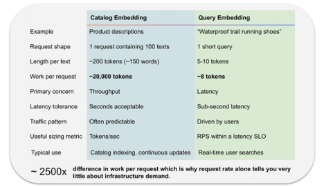
You're not running the same workload twice, you're asking one model to do two very different jobs. Infrastructure tuned for large batches won't necessarily deliver the same response times when serving thousands of small, latency-sensitive requests.
Reranking has a different request shape
Rerank workloads introduce another crucial variable into the mix: how many candidate documents you're actually asking the model to evaluate.
Let's stick with our product search example. First, your vector search might pull up 50 candidate products that match the query. Then the reranker steps in, it's like having a knowledgeable sales associate who looks at those 50 options and decides which ones truly deserve the top spots.
The model essentially compares the shopper's query against each candidate and ranks them by relevance. Each query-document pair is scored independently, which means the query gets processed once per candidate - so the work scales directly with how many candidates you send.
A typical rerank request looks like this: one short query of around 20 tokens, plus 50 candidate products at roughly 200 tokens each. That's about 11,000 tokens the model works through for a single search.
Simple enough, right? But here's where things get interesting. Suppose you change your strategy from reranking 20 candidates to 50 or 100. On the surface nothing changes for the user- same number of searches, same experience. Behind the scenes you've gone from about 4,400 tokens per search to about 22,000. It's the difference between asking someone to pick the best 20 products from a catalog versus ranking 100 of them. Same task, far more to read through.
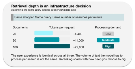
This is why retrieval depth becomes such a critical infrastructure decision. You're not just scaling based on user volume anymore, you're scaling based on how deep you want to dig into your results pool.
Traffic pattern matters as much as traffic volume
Once the request profile is understood, the next question is: How does traffic arrive?
Two applications can have the same peak traffic and still have very different infrastructure economics.
Sustained Traffic Patterns
Think about a global search service, traffic flows at a relatively consistent pace throughout the day. There's no drastic surge, no dramatic dips. In this scenario, dedicated capacity starts looking really attractive because your infrastructure stays nicely utilized. You're not paying for capacity that sits idle most of the time, and you're never scrambling to handle unexpected spikes.
Bursty Traffic Patterns
Now picture a different kind of application, maybe a financial reporting system or a batch processing job. This application maintains low traffic volume during standard operational periods, with concentrated spikes occurring during peak business hours or scheduled processing windows. For this scenario, consumption-based services are a good option because you're not paying for all that idle capacity during those low traffic volumes.
The real infrastructure question
It's not simply "How high is peak traffic?"
It's "How consistently can the infrastructure be utilized?"
Peak traffic tells you your maximum capacity needs, but utilization patterns tell you how efficiently you'll actually use that capacity. A service that handles 10,000 requests per second but only for 5 minutes a day has very different economics than one that handles 100 requests per second constantly. Getting this right means the difference between infrastructure that's just adequate and infrastructure that's truly optimal with respect to being cost-effective and responsive.
Beyond request volume: shape and pattern matter more
Looking only at request volume leads to poor infrastructure decisions. Consider these contrasting scenarios:
Low RPM, High Processing: A catalog embedding workload with just 30 requests per minute might seem small, but if each request contains 100 texts × 200 tokens, that's 600K tokens per minute of sustained processing. Dedicated capacity may be well-utilized.
High RPM, Low Processing: Thousands of query embedding requests per minute sounds demanding, but if each contains only a few tokens and traffic spikes last just hours, shared infrastructure may be more cost-effective.
Reranking follows the same pattern: Few searches with large candidate sets can outweigh many searches with small sets.
Key distinction:
- Request rate tells you how often the model is called
- Request shape tells you how much work each call represents
- Traffic patterns tell you how consistently capacity is needed
The cost crossover depends on the workload
Once request shape and traffic pattern are understood, you can estimate the point at which dedicated infrastructure becomes more economical than consumption-based inference. There is no universal break-even point, the crossover is specific to the workload.
For example, using the representative workloads and assumptions in this analysis:
**These break-evens are based on representative consumption-based pricing and a single dedicated NVIDIA A10 GPU instance billed hourly, assuming no negotiated discounts and traffic sustained 24×7. Workloads that run only part of the day require a higher request rate during active hours to reach the same economic crossover. A different instance type changes both cost and capacity, potentially shifting the break-even points. Instance throughput determines how much volume one instance can handle before additional capacity is required; it does not directly determine the economic crossover, which is based on pricing. Embedding is billed per token and reranking per search unit, so their request rates are not directly comparable. These figures are illustrative, workload-specific crossovers, not universal deployment thresholds.
The first three rows are the same model at the same price. The only thing that changes is the shape of the request, and the crossover moves from around four requests per minute to tens of thousands. A short query has to arrive in enormous volume before dedicated capacity is worth it. A batch of long documents gets there almost immediately.
That has a practical implication for the catalog workload described earlier. At 30 requests per minute it sounds like a small job, but the break-even for that exact request profile is ~20 requests per minute. It is already in the range where dedicated capacity is the more economical choice, despite the modest request rate.
Comparing across models needs more care. Embedding is billed per token and reranking per search unit, and their dedicated capacity costs differ, so ~20 and ~29 requests per minute aren't two points on the same scale. Reranking's crossover landing between the catalog and query profiles is a coincidence of these particular request shapes, not a property of the models.
Change the compute capacity, the pricing model, or the utilization pattern and the break even point changes.
Latency changes the equation
Maximum throughput doesn't equal usable capacity because different workloads have fundamentally different performance requirements.
- Batch indexing: Can operate at peak throughput since completion efficiency matters more than immediate response
- Search queries: Require strict latency targets - response time directly impacts user experience and business outcomes
- Reranking: Expanding candidate sets improves documents/sec processed while lowering the searches/sec served
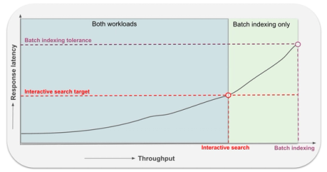
This latency-throughput trade-off means infrastructure sizing must account for both performance dimensions. For interactive workloads, capacity should be based on sustainable throughput that meets target latency requirements, not just maximum benchmark performance. This often necessitates additional headroom beyond peak demand calculations.
One simple decision framework
Before choosing shared or dedicated inference for Embed or Rerank, answer these questions and the infrastructure decision becomes much easier
Takeaway
When people start comparing shared and dedicated inference, they usually reach for two numbers first, the price per token and the requests per minute. Neither one really tells you much on its own. What you actually want to know is how much work each request is carrying, how steadily it shows up, and whether your capacity is going to stay busy.
So there's no magic break-even number to look up. The crossover belongs to your workload, not to the deployment option you picked. And many search applications end up using both, dedicated capacity for the catalog indexing and consumption pricing for the query traffic that spikes based on end user demand.
Understand the request → Understand the traffic → Understand the utilization → Then pick the deployment model.